Constructing twpas#

This tutorial shows how to define and customize a TWPA model. At the moment, twpasolver is specialized to model KI-TWPAS only, but new components modeling the reposne of Josephson Junctions can be easily implemented.

Using predefined models#

Let’s start by defining some parameters for the cells of the device. We consider a simple design with step modulation between a certain number of loaded and an unloaded cells. We also define the circuit parameters for a mean effective TWPA without modulation, and compare the response of the devices.

[1]:

import matplotlib.pyplot as plt
import numpy as np
from numba import njit

from twpasolver.frequency import Frequencies
from twpasolver.models import TWPA, LCLfBaseCell, StubBaseCell

freqs = np.arange(1e9, 12e9, 2e6)
N_u = 60
N_l = 6
N_sc = 1000
N = N_sc * (N_u + N_l)

# Cell capacitances, expressed in F
C_u = 18.81e-15
C_l = 7.0e-15
C_eff = (N_u * C_u + N_l * C_l) / (N_u + N_l)

# Cell inductances, expressed in H
L_u = 45.2e-12
L_l = 45.2e-12
L_eff = (N_u * L_u + N_l * L_l) / (N_u + N_l)

# Finger inductances, expressed in H
L_f_u = 1.02e-9
L_f_l = 0.335e-9
L_f_eff = (N_u * L_f_u + N_l * L_f_l) / (N_u + N_l)

# Characteristic inductance
Z_0 = np.sqrt(L_u / C_u)
Z_l = np.sqrt(L_l / C_l)
Z_eff = np.sqrt(L_eff / C_eff)

l1_u = 102e-6
l1_l = 33.5e-6
l2 = 2e-6

We can now define the models for the cells and TWPAs. The twpasolver.models.TWPA class is derived from twpasolver.models.TwoPortArray, with additional arguments to represent the parameters of the nonlinear response, which will be used to find the phase-matching condition and the gain profile in the next tutorial. The LCLfBaseCell model determines the single cell response as detailed in Appendix B of 10.1103/PRXQuantum.

[2]:

unloaded = LCLfBaseCell(C=C_u, L=L_u, Lf=L_f_u, N=N_u / 2)
loaded = LCLfBaseCell(C=C_l, L=L_l, Lf=L_f_l, N=N_l)
twpa = TWPA(cells=[unloaded, loaded, unloaded], N=N_sc)

# Effective mean cell and unmodulated TWPA
eff = LCLfBaseCell(C=C_eff, L=L_eff, Lf=L_f_eff, N=N_u + N_l)
twpa_not_loaded = TWPA(cells=[eff], N=N_sc)

twpa.model_dump()

[2]:

{'Z0_ref': 50.0,
 'N': 1000,
 'cells': [{'Z0_ref': 50.0,
   'N': 30,
   'name': 'LCLfBaseCell',
   'L': 4.52e-11,
   'C': 1.881e-14,
   'Lf': 1.02e-09,
   'delta': 0.0,
   'centered': False},
  {'Z0_ref': 50.0,
   'N': 6,
   'name': 'LCLfBaseCell',
   'L': 4.52e-11,
   'C': 7e-15,
   'Lf': 3.35e-10,
   'delta': 0.0,
   'centered': False},
  {'Z0_ref': 50.0,
   'N': 30,
   'name': 'LCLfBaseCell',
   'L': 4.52e-11,
   'C': 1.881e-14,
   'Lf': 1.02e-09,
   'delta': 0.0,
   'centered': False}],
 'name': 'TWPA',
 'Istar': 0.0065,
 'Idc': 0.001,
 'Ip0': 0.0002,
 'N_tot': 66000,
 'epsilon': 46.242774566474,
 'xi': 23121.387283236996,
 'chi': 0.00011560693641618498,
 'alpha': 1.0236686390532543,
 'Iratio': 0.15384615384615385}

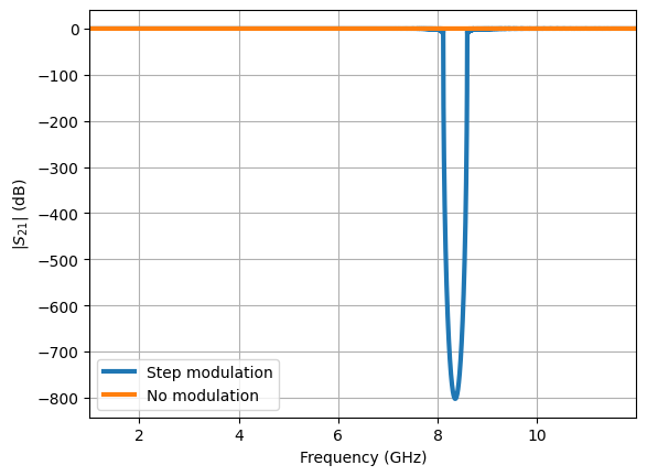
As usual, we plot the response of the devices, starting from the magnitude of \(S_{21}\). The cell modulation creates a stopband.

[3]:

net = twpa.get_network(freqs)
net_unmodulated = twpa_not_loaded.get_network(freqs)

net.s21.plot_s_db(label="Step modulation", lw=3)
net_unmodulated.s21.plot_s_db(label="No modulation", lw=3)
plt.ylabel("$|S_{21}|$ (dB)")
plt.grid()

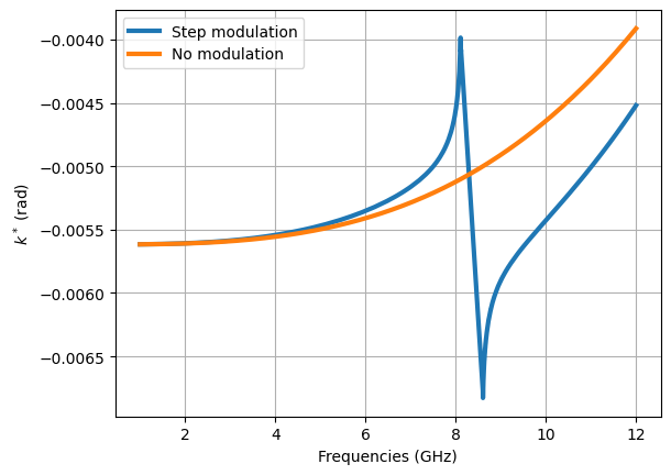
Another important aspect of the response of a TWPA is the nonlinear dependence of the phase of \(S_{21}\). The modulation creates a resonance-like profile that restricts the phase matching condition to a controllable range.

[4]:

linear_disp = 2 * np.pi * freqs * np.sqrt(C_eff * L_eff)
plt.plot(
    freqs * 1e-9,
    -net.s21.s_rad_unwrap.flatten() / N - linear_disp,
    label="Step modulation",
    lw=3,
)
plt.plot(
    freqs * 1e-9,
    -net_unmodulated.s21.s_rad_unwrap.flatten() / N - linear_disp,
    label="No modulation",
    lw=3,
)
plt.xlabel("Frequencies (GHz)")
plt.ylabel("$k^*$ (rad)")
plt.legend()
plt.grid()

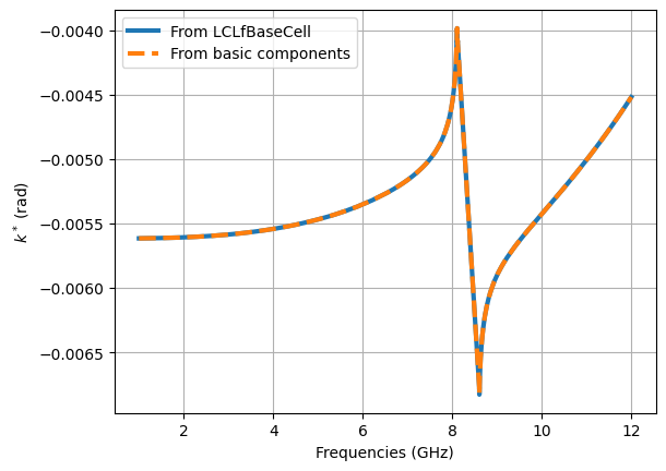
Constructing models from basic components#

It is also possible to explicitly use the composition of basic circuit elements to generate a TWPA. Here’s how to repoduce the LCLfBaseCell model starting from inductors and capacitors.

[5]:

from twpasolver.models import Capacitance, Inductance, compose

L_line_u = Inductance(L=L_u)
fingers_u = compose(
    Capacitance(C=C_u / 2), Inductance(L=L_f_u), N=2, twoport_parallel=True
)
cell_u = compose(L_line_u, fingers_u, N=N_u / 2)

L_line_l = Inductance(L=L_l)
fingers_l = compose(
    Capacitance(C=C_l / 2), Inductance(L=L_f_l), N=2, twoport_parallel=True
)
cell_l = compose(L_line_l, fingers_l, N=N_l)

twpa_from_basic = TWPA(cells=[cell_u, cell_l, cell_u], N=N_sc)

# Plot the nonlinear phase response
plt.plot(
    freqs * 1e-9,
    -net.s21.s_rad_unwrap.flatten() / N - linear_disp,
    label="From LCLfBaseCell",
    lw=3,
)
plt.plot(
    freqs * 1e-9,
    -twpa_from_basic.get_network(freqs).s21.s_rad_unwrap.flatten() / N - linear_disp,
    label="From basic components",
    lw=3,
    ls="--",
)
plt.xlabel("Frequencies (GHz)")
plt.ylabel("$k^*$ (rad)")
plt.legend()
plt.grid()